Chainer at a Glance
Welcome to Chainer!
Chainer is a rapidly growing neural network platform. The strengths of Chainer are:
Python-based – Chainer is developed in Python, allowing for inspection and customization of all code in python and understandable python messages at run time
Define by Run – neural networks definitions are defined on-the-fly at run time, allowing for dynamic network changes
NumPy based syntax for working with arrays, thanks to CuPy implementation
Fully customizable – since Chainer is pure python, all classes and methods can be adapted to allow for the latest cutting edge or specialized approaches
Broad and deep support – Chainer is actively used for most of the current approaches for neural nets (CNN, RNN, RL, etc.), aggressively adds new approaches as they’re developed, and provides support for many kinds of hardware as well as parallelization for multiple GPUs
Mushrooms – tasty or deadly?
Let’s take a look at a basic program of Chainer to see how it works. For a dataset, we’ll work with Kaggle’s edible vs. poisonous mushroom dataset, which has over 8,000 examples of mushrooms, labelled by 22 categories including odor, cap color, habitat, etc., in a mushrooms.csv file.
How will Chainer learn which mushrooms are edible and which mushrooms will kill you? Let’s see!
The code below is from the glance example in the examples/glance directory.
Code Breakdown
Initialization
Let’s start the program. Here are the typical imports for a Chainer program. chainer.links contain trainable parameters and chainer.functions do not.
 6import chainer as ch
 7from chainer import datasets
 8import chainer.functions as F
 9import chainer.links as L
10from chainer import training
11from chainer.training import extensions
12
13import numpy as np
We’ll use Matplotlib for the graphs to show training progress.
15import matplotlib
16matplotlib.use('Agg')
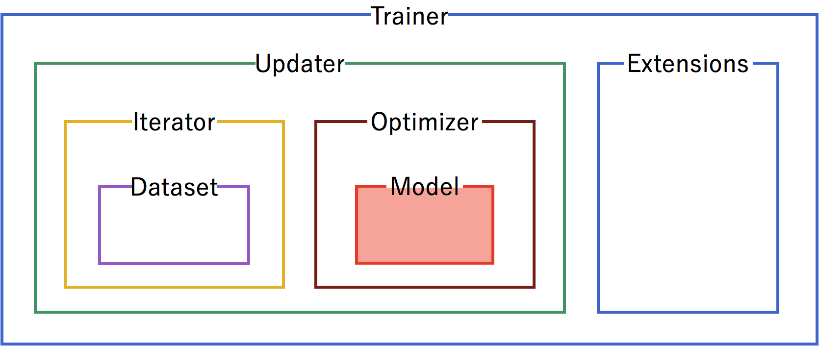
Trainer Structure
A trainer is used to set up our neural network and data for training. The components of the trainer are generally hierarchical, and are organized as follows:
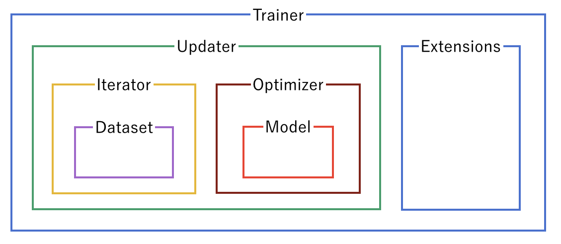
Each of the components is fed information from the components within it. Setting up the trainer starts at the inner components, and moves outward, with the exception of extensions, which are added after the trainer is defined.
Dataset
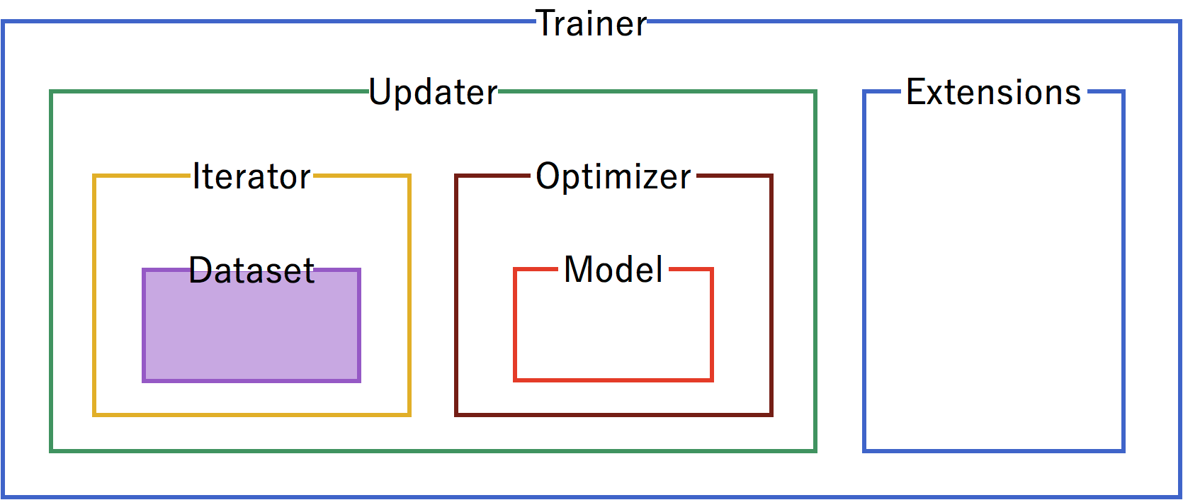
Our first step is to format the dataset. From the raw mushrooms.csv, we format the data into a Chainer TupleDataset.
18mushroomsfile = 'mushrooms.csv'
19data_array = np.genfromtxt(
20    mushroomsfile, delimiter=',', dtype=str, skip_header=1)
21for col in range(data_array.shape[1]):
22    data_array[:, col] = np.unique(data_array[:, col], return_inverse=True)[1]
23
24X = data_array[:, 1:].astype(np.float32)
25Y = data_array[:, 0].astype(np.int32)[:, None]
26train, test = datasets.split_dataset_random(
27    datasets.TupleDataset(X, Y), int(data_array.shape[0] * .7))
Iterator
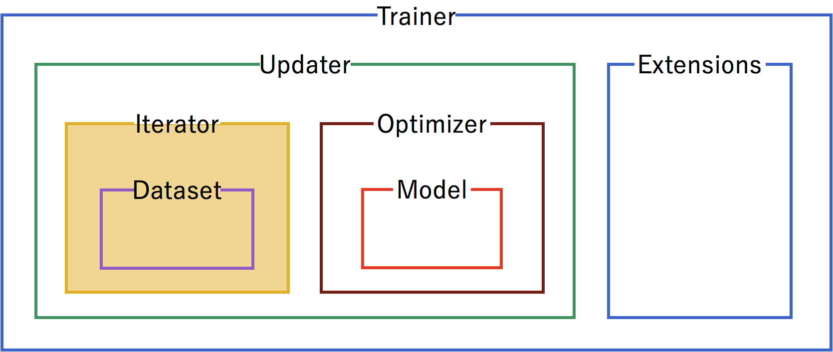
Configure iterators to step through batches of the data for training and for testing validation. In this case, we’ll use a batch size of 100. For the training iterator, repeating and shuffling are implicitly enabled, while they are explicitly disabled for the testing iterator.
29train_iter = ch.iterators.SerialIterator(train, 100)
30test_iter = ch.iterators.SerialIterator(
31    test, 100, repeat=False, shuffle=False)
Model
Next, we need to define the neural network for inclusion in our model. For our mushrooms, we’ll chain together two fully-connected, Linear, hidden layers between the input and output layers.
As an activation function, we’ll use standard Rectified Linear Units (relu()).
Using Sequential allows us to define the neural network model in a compact format.
34# Network definition
35def MLP(n_units, n_out):
36    layer = ch.Sequential(L.Linear(n_units), F.relu)
37    model = layer.repeat(2)
38    model.append(L.Linear(n_out))
39
40    return model
Since mushrooms are either edible or poisonous (no information on psychedelic effects!) in the dataset, we’ll use a Link Classifier for the output, with 44 units (double the features of the data) in the hidden layers and a single edible/poisonous category for classification.
43model = L.Classifier(
44    MLP(44, 1), lossfun=F.sigmoid_cross_entropy, accfun=F.binary_accuracy)
Note that in the two code snippets above we have not specified the size of the input layer. Once we start feeding the neural network with samples, Chainer will recognize the dimensionality of the input automatically and initialize the matrix for each layer with the appropriate shape. In the example above, that is 44×22 for the first hidden layer, 44×44 for the second hidden layer, and 1×44 for the output layer.
Optimizer
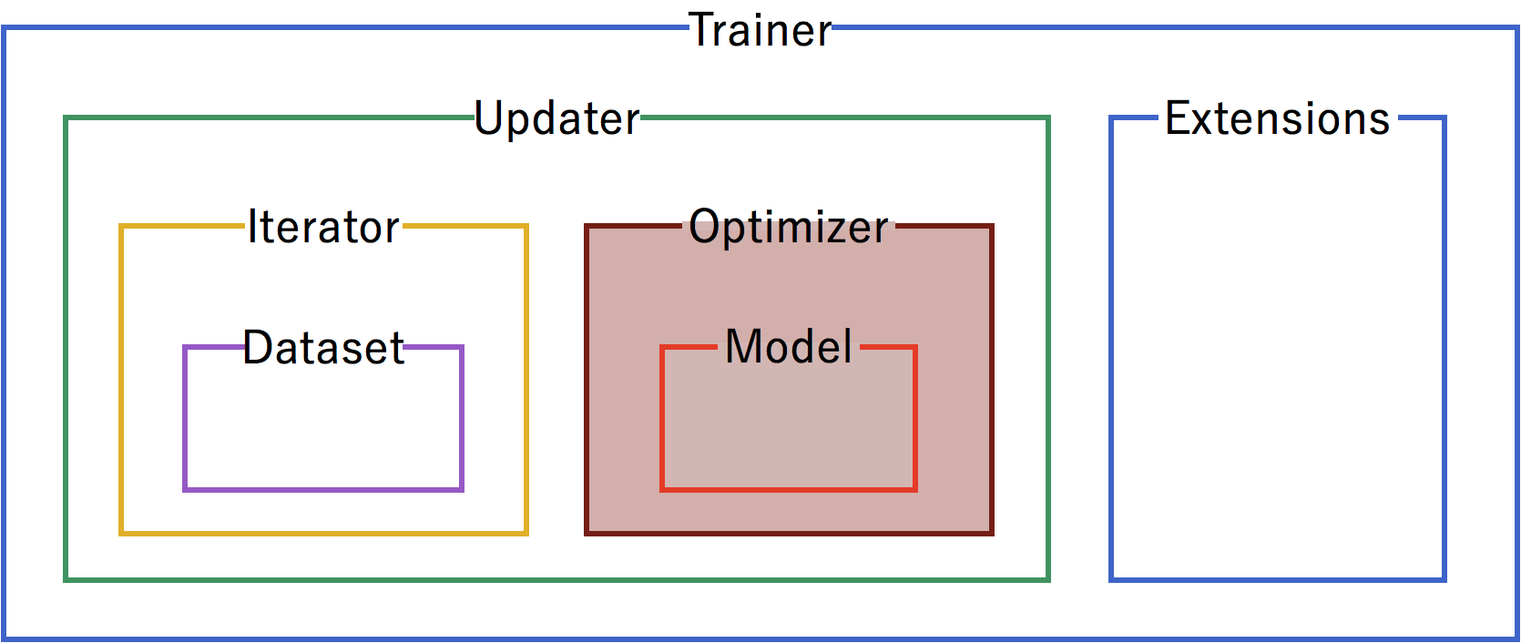
Pick an optimizer, and set up the model to use it.
46# Setup an optimizer
47optimizer = ch.optimizers.SGD().setup(model)
Updater

Now that we have the training iterator and optimizer set up, we link them both together into the updater. The updater uses the minibatches from the iterator, does the forward and backward processing of the model, and updates the parameters of the model according to the optimizer. Setting the device=-1 sets the device as the CPU. To use a GPU, set device equal to the number of the GPU, usually device=0.
49# Create the updater, using the optimizer
50updater = training.StandardUpdater(train_iter, optimizer, device=-1)
Finally we create a Trainer object. The trainer processes minibatches using the updater defined above until a certain stop condition is met and allows the use of extensions during the training. We set it to run for 50 epochs and store all files created by the extensions (see below) in the result directory.
52# Set up a trainer
53trainer = training.Trainer(updater, (50, 'epoch'), out='result')
Extensions
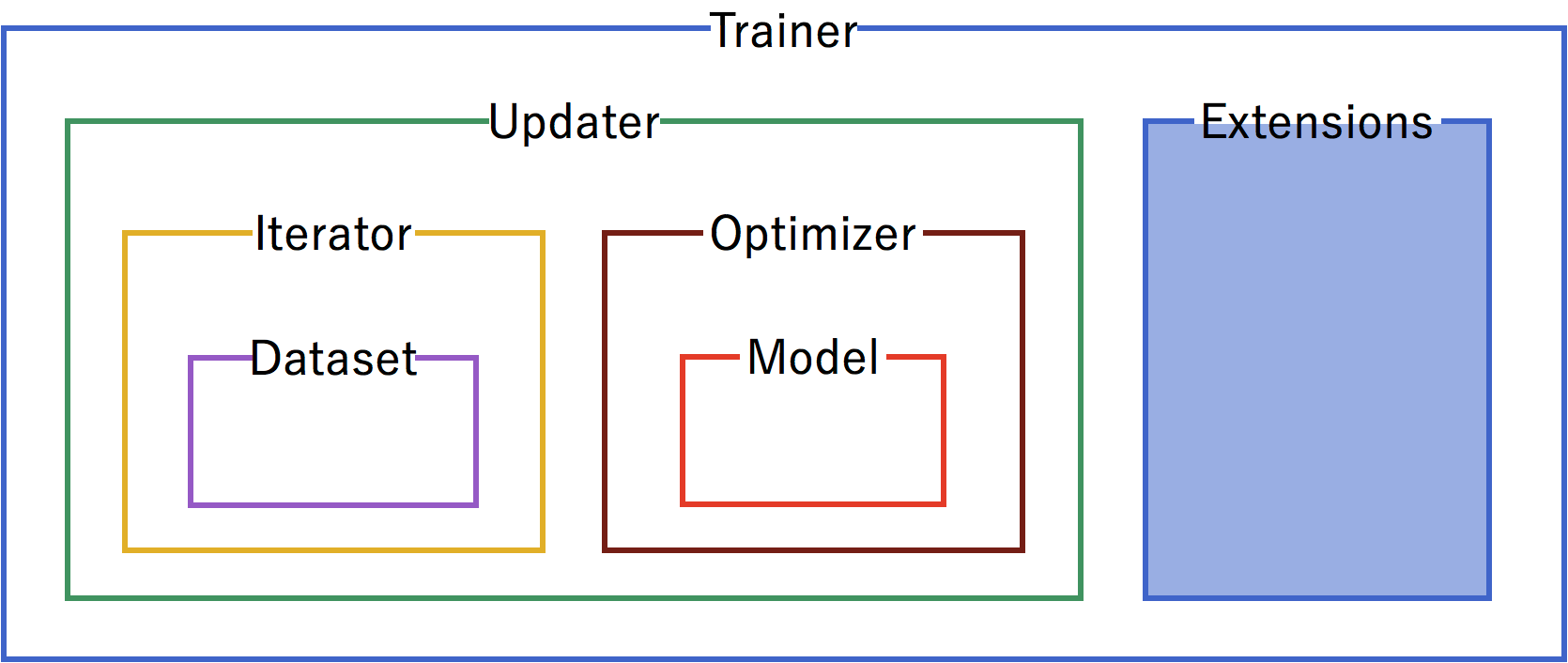
Extensions can be used to execute code at certain events during the training, such as every epoch or every 1000 iterations. This mechanism is used in Chainer to evaluate models during training, print progress messages, or dump intermediate model files.
First, use the testing iterator defined above for an Evaluator extension to the trainer to provide test scores. If using a GPU instead of the CPU, set device to the ID of the GPU, usually 0.
54# Evaluate the model with the test dataset for each epoch
55trainer.extend(extensions.Evaluator(test_iter, model, device=-1))
Save a computational graph from loss variable at the first iteration. main refers to the target link of the main optimizer. The graph is saved in the Graphviz’s dot format. The output location (directory) to save the graph is set by the out argument of trainer.
57# Dump a computational graph from 'loss' variable at the first iteration
58# The "main" refers to the target link of the "main" optimizer.
59trainer.extend(extensions.DumpGraph('main/loss'))
Take a snapshot of the trainer object every 20 epochs.
61trainer.extend(extensions.snapshot(), trigger=(20, 'epoch'))
Write a log of evaluation statistics for each epoch.
63# Write a log of evaluation statistics for each epoch
64trainer.extend(extensions.LogReport())
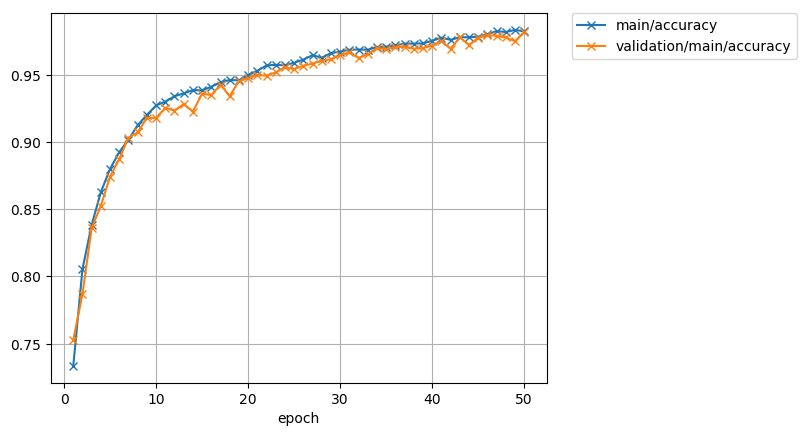
Save two plot images to the result directory.
66# Save two plot images to the result dir
67trainer.extend(
68    extensions.PlotReport(['main/loss', 'validation/main/loss'],
69                          'epoch', file_name='loss.png'))
70trainer.extend(
71    extensions.PlotReport(
72        ['main/accuracy', 'validation/main/accuracy'],
73        'epoch', file_name='accuracy.png'))
Print selected entries of the log to standard output.
75# Print selected entries of the log to stdout
76trainer.extend(extensions.PrintReport(
77    ['epoch', 'main/loss', 'validation/main/loss',
78     'main/accuracy', 'validation/main/accuracy', 'elapsed_time']))
Main Loop
Finally, with the trainer and all the extensions set up, we can add the line that actually starts the main loop:
80#  Run the training
81trainer.run()
Inference
Once the training is complete, only the model is necessary to make predictions. Let’s check that a random line from the test data set and see if the inference is correct:
83x, t = test[np.random.randint(len(test))]
84
85predict = model.predictor(x[None]).array
86predict = predict[0][0]
87
88if predict >= 0:
89    print('Predicted Poisonous, Actual ' + ['Edible', 'Poisonous'][t[0]])
90else:
91    print('Predicted Edible, Actual ' + ['Edible', 'Poisonous'][t[0]])
Output
Output for this instance will look like:
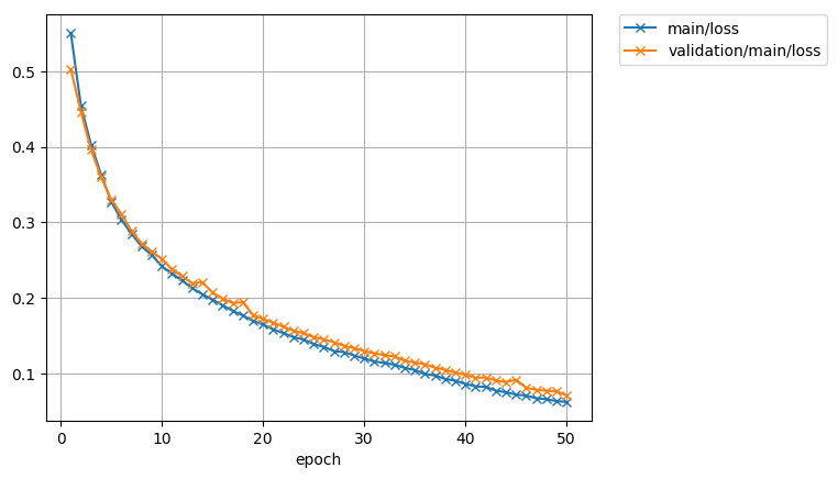
epoch       main/loss   validation/main/loss  main/accuracy  validation/main/accuracy  elapsed_time
1           0.550724    0.502818              0.733509       0.752821                  0.215426
2           0.454206    0.446234              0.805439       0.786926                  0.902108
3           0.402783    0.395893              0.838421       0.835979                  1.50414
4           0.362979    0.359988              0.862807       0.852632                  2.24171
5           0.32713     0.329881              0.88           0.874232                  2.83247
6           0.303469    0.31104               0.892456       0.887284                  3.45173
7           0.284755    0.288553              0.901754       0.903284                  3.9877
8           0.26801     0.272033              0.9125         0.907137                  4.54794
9           0.25669     0.261355              0.920175       0.917937                  5.21672
10          0.241789    0.251821              0.927193       0.917937                  5.79541
11          0.232291    0.238022              0.93           0.925389                  6.3055
12          0.222805    0.22895               0.934035       0.923389                  6.87083
13          0.21276     0.219291              0.93614        0.928189                  7.54113
14          0.204822    0.220736              0.938596       0.922589                  8.12495
15          0.197671    0.207017              0.938393       0.936042                  8.69219
16          0.190285    0.199129              0.941053       0.934842                  9.24302
17          0.182827    0.193303              0.944386       0.942695                  9.80991
18          0.176776    0.194284              0.94614        0.934042                  10.3603
19          0.16964     0.177684              0.945789       0.945242                  10.8531
20          0.164831    0.171988              0.949825       0.947347                  11.3876
21          0.158394    0.167459              0.952982       0.949747                  11.9866
22          0.153353    0.161774              0.956964       0.949347                  12.6433
23          0.148209    0.156644              0.957368       0.951747                  13.3825
24          0.144814    0.15322               0.957018       0.955495                  13.962
25          0.138782    0.148277              0.958947       0.954147                  14.6
26          0.135333    0.145225              0.961228       0.956695                  15.2284
27          0.129593    0.141141              0.964561       0.958295                  15.7413
28          0.128265    0.136866              0.962632       0.960547                  16.2711
29          0.123848    0.133444              0.966071       0.961347                  16.7772
30          0.119687    0.129579              0.967193       0.964547                  17.3311
31          0.115857    0.126606              0.968596       0.966547                  17.8252
32          0.113911    0.124272              0.968772       0.962547                  18.3121
33          0.111502    0.122548              0.968596       0.965095                  18.8973
34          0.107427    0.116724              0.970526       0.969747                  19.4723
35          0.104536    0.114517              0.970877       0.969095                  20.0804
36          0.099408    0.112128              0.971786       0.970547                  20.6509
37          0.0972982   0.107618              0.973158       0.970947                  21.2467
38          0.0927064   0.104918              0.973158       0.969347                  21.7978
39          0.0904702   0.101141              0.973333       0.969747                  22.3328
40          0.0860733   0.0984015             0.975263       0.971747                  22.8447
41          0.0829282   0.0942095             0.977544       0.974947                  23.5113
42          0.082219    0.0947418             0.975965       0.969347                  24.0427
43          0.0773362   0.0906804             0.977857       0.977747                  24.5252
44          0.0751769   0.0886449             0.977895       0.972147                  25.1722
45          0.072056    0.0916797             0.978246       0.977495                  26.0778
46          0.0708111   0.0811359             0.98           0.979347                  26.6648
47          0.0671919   0.0783265             0.982456       0.978947                  27.2929
48          0.0658817   0.0772342             0.981754       0.977747                  27.8119
49          0.0634615   0.0762576             0.983333       0.974947                  28.3876
50          0.0622394   0.0710278             0.982321       0.981747                  28.9067
Predicted Edible Actual Edible
Our prediction was correct. Success!
The loss function:
And the accuracy